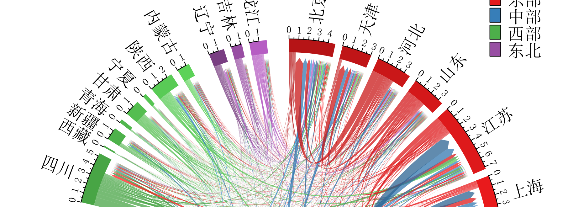
R code for chord diagrams of Chinese internal migration

We have had a number of requests for the R code to replicate the plots in our paper on internal migration in China. The code below will produce a similar looking plot, but I have taken out some of the arguments that were very specific to our plot that will not replicate well for other data.

Data

The code is based on two data sets:

1. Bilateral flow data with three columns only (origin, destination and flow), see here for the file used below
2. Region details used for plotting, see here for the file used below

Note, the names in the region data are the same as the ones used in the origin and destination data.

We can read in the data using read_csv() in the readr package

library(tidyverse)

d1 <- read_csv("https://gist.githubusercontent.com/guyabel/c24d990abc2c692f2b63747ee42909eb/raw/6b255edee7e01ca31b856152d18ae10ad50badd5/china_flow_2010_2015.csv")

d1 <- mutate(d1, flow = flow/1e6)
d1

## # A tibble: 961 x 3
##    orig           dest      flow
##    <chr>          <chr>    <dbl>
##  1 Beijing        Beijing 0     
##  2 Tianjin        Beijing 0.0674
##  3 Hebei          Beijing 0.864 
##  4 Shanxi         Beijing 0.225 
##  5 Inner Mongolia Beijing 0.103 
##  6 Liaoning       Beijing 0.155 
##  7 Jilin          Beijing 0.105 
##  8 Heilongjiang   Beijing 0.194 
##  9 Shanghai       Beijing 0.0266
## 10 Jiangsu        Beijing 0.111 
## # ... with 951 more rows

d2 <- read_csv("https://gist.githubusercontent.com/guyabel/2f52e1593ad951800d83530a58ce0079/raw/165843fdd4afc61e17cd7658563e573c1e74fb57/china_region_details.csv")
d2

## # A tibble: 31 x 6
##    name      region order colour    gap name_zh
##    <chr>     <chr>  <dbl> <chr>   <dbl> <chr>  
##  1 Beijing   East       1 #B61416     2 <U+5317><U+4EAC>   
##  2 Tianjin   East       2 #C01517     2 <U+5929><U+6D25>   
##  3 Hebei     East       3 #CA1718     2 <U+6CB3><U+5317>   
##  4 Shandong  East       4 #D4181A     2 <U+5C71><U+4E1C>   
##  5 Jiangsu   East       5 #DE191B     2 <U+6C5F><U+82CF>   
##  6 Shanghai  East       6 #E91A1C     2 <U+4E0A><U+6D77>   
##  7 Zhejiang  East       7 #F31B1D     2 <U+6D59><U+6C5F>   
##  8 Fujian    East       8 #FD1C1F     2 <U+798F><U+5EFA>   
##  9 Guangdong East       9 #FF1E20     2 <U+5E7F><U+4E1C>   
## 10 Hainan    East      10 #FF1F21     6 <U+6D77><U+5357>   
## # ... with 21 more rows

Plot

The code below plots the chord diagram without the default labels and axis for the chordDiagram() function, that are added later in the circos.track() function.

library(circlize)

circos.clear()
circos.par(track.margin = c(0.01, -0.01), start.degree = 90, gap.degree = d2$gap)

chordDiagram(x = d1, order = d2$name, 
             grid.col = d2$colour, transparency = 0.25,
             directional = 1, direction.type = c("diffHeight", "arrows"),
             link.arr.type = "big.arrow", diffHeight = -0.04, 
             link.sort = TRUE, link.largest.ontop = TRUE, 
             annotationTrack = "grid",
             preAllocateTracks = list(track.height = 0.25))

circos.track(track.index = 1, bg.border = NA, panel.fun = function(x, y) {
  s = get.cell.meta.data("sector.index")
  xx = get.cell.meta.data("xlim")
  circos.text(x = mean(xx), y = 0.2, 
              labels = s, cex = 0.7, adj = c(0, 0.5),
              facing = "clockwise", niceFacing = TRUE)
  circos.axis(h = "bottom",
              labels.cex = 0.5,
              labels.pos.adjust = FALSE,
              labels.niceFacing = FALSE)
})

The legend is added using the legend() function using the Set1 colour palette, that we used as the basis of regional shades in the colour column of d2; see the shades package for creating palettes of similar colours.

Legend

library(RColorBrewer)
legend(x = 0.7, y = 1.1, 
       legend = unique(d2$region), 
       fill = brewer.pal(n = 4, name = "Set1"), 
       bty = "n", cex = 0.8,
       x.intersp = 0.5, 
       title = "   Region", title.adj = 0) 

Saving

To save the image in a PDF plot surround the plotting code above between the pdf() function and dev.off() function.

pdf(file = "figure1.pdf", width = 6, height = 6)

### insert code from above

dev.off()

Image Files

To convert the PDF to a PNG file I recommend the magick package:

library(magick)
p <- image_read_pdf("figure1.pdf")
image_write(image = p, path = "figure1.png")

Chinese Labels

To replace the labels with their Chinese names, as in the plot above, replace the code for the s object in the circos.track() function to:

    s = d2 %>% 
      filter(name == get.cell.meta.data("sector.index")) %>%
      select(name_zh) %>%
      pull()

You might also need to add family = "GB1" in the pdf() function for Chinese characters to render in a PDF viewer.