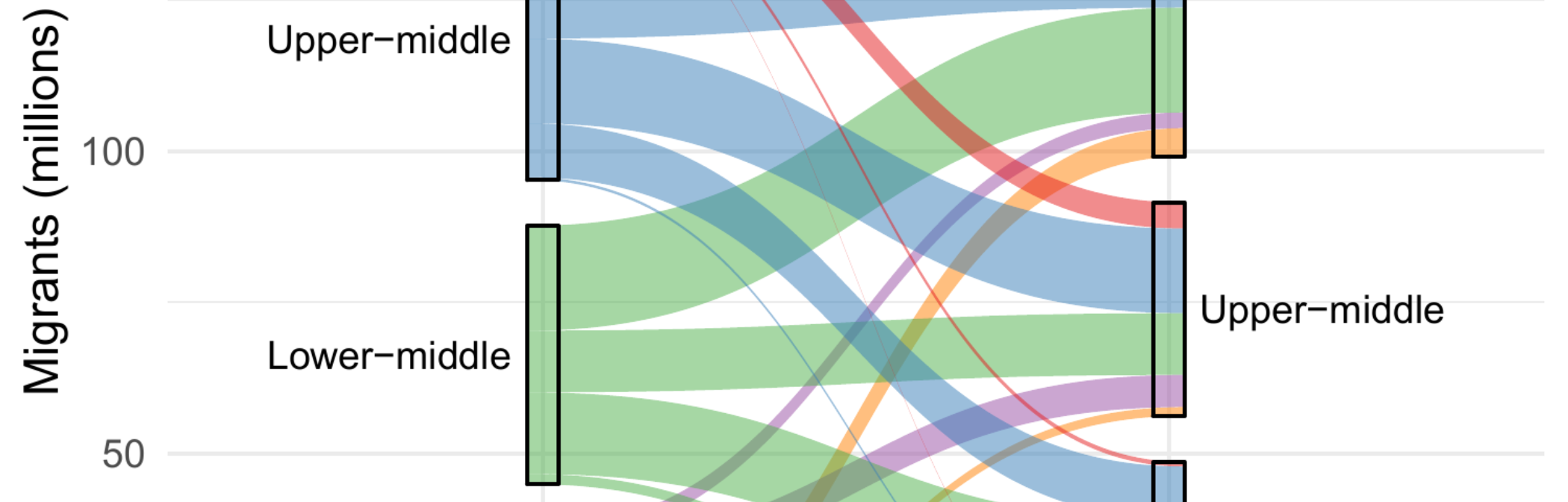
Animated Sankey plots of global migrant populations

Background

Sankey plots have been used to visualize bilateral migration many times. My favorite examples of Sankey plots for migration data tend to be when there are only few regions or countries. As the number of regions or countries increases the plot become more cumbersome, where labels for the smaller areas get too small and the plotting area becomes a very long rectangle making it awkward to fit on paper or view on the screen. In such cases I prefer chord diagrams

The recent highlights document for the UN international migration stock data contained a couple of Sankey plots for the data in 2020. In this post I have created animated versions of one of the plots in the report to show changes in migrant distributions between 1990 and 2020 by World Bank income groups. I am using the destination and origin migrant stock data of the UN that can found online here - see the data links on the right hand side.

R Code

Commented code to create the animated plots below are in a Gist here. You can run the script directly in R using the following…

library(devtools)
source_gist("https://gist.github.com/guyabel/f7c844f18c4d11916a6ee000532d0e8e")

…so long as you have installed all packages used in the script. You might also need to edit the saveVideo() function for the location of ffmpeg.exe.

The first part of the code imports the data into R, extracts the rows for the stock data by the World Bank income groups and creates a tweened data set for each frame of the animation.

The second part of the code creates the animated plot file using ggplot and geom_parallel_sets() in ggforce. There are a few packages in R that have functions for Sankey plots, for example sankey, PantaRhei, networkD3, sankeywheel, plotly and ggsankey. The ggalluvial packages also produces Sankey-type plots, but without spaces between each sector. I used ggforce because it is pretty easy to tweak the non-Sankey parts of the plot using ggplot functions, and I had hoped that it would play well with gganimate - which it didn’t, hence the use of tweenr - but perhaps one day it will.

Plots

The first animated plot shows the changes over time where the y-axis increases as the migrant populations grow larger. It shows the evolution in the relative distributions of the origin, destination and the linking migrant corridors, in particular the relative growth of migrants in high income countries.

Note: you might have to right click, select show controls and hit play to start the animations depending on your browsers - right clicking can also allow you to access controls on the play back speed and save the video if you want to use it elsewhere.

The second animated plot shows the changes over time where the y-axis is fixed to its maximum level. The adjustment allows the Sankey to grow into the plot space to see more clearly the changes in the overall levels of migrant populations.

For both plots above there are alternative versions, that include an additional origin category for unknown place of birth. The values for the stock of migrants with unknown origins living in each World Bank income group are not in the main data frame in the UN excel sheet, but are in the regional aggregate sheets for each period. As a result the data importing and manipulation takes a bit of extra work (it is commented out in the Gist R script), but the plots are more ‘complete’, where the totals of the sectors sum to the global estimate of the UN at each time point.